Abstract
Stablecoins are commonly classified according to their issuers’ stated design, such as fiat-backed, crypto-backed, or algorithmic. This note examines whether stablecoins also sort into discrete behavioral types based on observed conduct. We compute six behavioral measures, one for each construct, for 111 stablecoins that survived and had adequate price and issuance data over the first 180 days after first sustaining $1 million in the issuance record. No observations after day 179 enter the analysis, so subsequent outcomes cannot affect the measurement window.
Three rotated principal components explain 95% of the variance and capture local peg stability, supply trajectory, defined by growth relative to drawdown, and supply volatility. We test whether this component space contains discrete groups using an explicitly stated decision rule calibrated against simulated samples of the same size, including 2,000 draws from a Gaussian-copula continuum that preserves the empirical marginals and planted three-group mixtures with known separation.
The observed data do not satisfy the rule for discrete types. Cluster separation remains within the continuum reference range at every partition size, the overlap-penalized mixture criterion selects a single component, and the only partition whose bootstrap reproducibility exceeds the continuum reference corresponds to a supply tail that is not corroborated by either the separation measures or the mixture criteria. The rule has a 0.2% false-positive rate under the continuum. It detects planted groups separated by four standard deviations of the leading component in 99% of simulations and groups separated by three standard deviations in 14%.
Declared backing category is associated with a small shift in behavioral position. In the fiat-backed versus crypto-backed comparison, backing category explains 4% of score variance (permutation p = 0.006), while a separate dispersion test does not reject equal dispersion (p = 0.84). Fiat-backed coins are more stable around local par and exhibit less drawdown and stronger supply growth over the first six months. Behavioral measures also predict the two backing labels modestly better than chance out of fold, with balanced accuracy of 0.64 against a chance benchmark of 0.50.
Among well-documented stablecoins that survive a common early-life window, these methods identify no behavioral partition that is jointly more separated, better supported by mixture criteria, and more stable than calibrated continuum references. This note accompanies a separate survival analysis of stablecoin mortality currently in preparation.
Keywords: stablecoins, cluster analysis, principal components, behavioral classification, calibration, negative results.
JEL classification: E42, G23, C38.
1. The question
Taxonomies of stablecoins in current use sort coins by design. Central-bank and supervisory work classifies by the nature of the backing claim and its custody: tokenized funds, off-chain and on-chain collateralized coins, and algorithmic designs (Bullmann, Klemm and Pinna, 2019); by the regulatory perimeter the claim falls under (Arner, Auer and Frost, 2020); or by the source and management of collateral, with stability examined by design type (Hafner, Henriques Pereira, Dietl and Beccuti, 2024). Empirical work on instability asks which design features and market conditions precede depegs (Kwon, Pongmala, Qin, Klages-Mundt, Jovanovic, Parlour, Gervais and Song, 2023) and how survival and transaction costs differ across coins (Mizrach, 2025). Two studies have asked whether measured conduct agrees with design. Gadzinski, Castello and Mazzorana (2023) apply community detection to stablecoin price dynamics and find clusters broadly in line with protocol types, with exceptions in which non-custodial and algorithmic coins move like established custodial ones. Song (2026) applies deep temporal clustering to rolling trajectories of exchange-rate-adjusted peg deviations for 18 stablecoins and finds two behavioral regimes, distinguished mainly by upper-tail behavior, that correspond only weakly to the coins' reference-currency labels; the regimes are read as descriptive rather than as asset classes. Both studies work on price alone and take the partition their algorithm returns as the object of study. This note asks a prior question and supplies a reference for it: whether the space of measured conduct, over a window common to every coin and on supply as well as price, falls into discrete regions at all, judged against what the same procedure returns on a continuum of the same size and shape, with a measured false-positive rate and power; and whether the declared backing category occupies a distinct region of that space.
The question has a statistical form. Take a set of behavioral measurements that owe nothing to the declared design, place each coin in the space they define, and ask two things: does the space contain discrete groups, and do the declared categories occupy distinct regions of it. Both questions need a reference. Partitioning algorithms such as k-means always return a partition; only a comparison with what the same algorithm returns on a continuum of the same size and shape says whether the partition means anything. This note supplies that comparison and states explicitly what counts as groups in the reported decision rule.
The population is narrower than "stablecoins". Every coin here survived its first six months and was observed with adequate coverage through them; a type of coin that fails faster than that cannot appear in the analysis, and a 90-day window is reported to show how much that conditioning matters (Appendix B).
2. Data
2.1 Origin and window
Each coin's origin is the first day of a seven-day run with at least $1 million of circulating supply, the birth clock of the companion mortality paper. Every measurement in this note is taken on days 0 to 179 after origin; nothing after day 179 and nothing before day 0 is read, including by the rolling par estimator described below. A coin that later collapsed and a coin that later thrived are measured on the same terms. Windows of 90 and 365 days are reported as sensitivities.
The origin is a property of the issuance record, not a launch date. For 70 of the 111 primary coins the origin is the first day the record carries the coin at all, and 47% enter the record already above $10 million (16% above $50 million). Some of these are genesis mints that reached size on their first day; others were in circulation before the record began. The two cannot be told apart without curated launch dates, which this note does not have. Two rules limit the exposure. A coin whose market price predates its observed origin by more than 90 days was certainly in circulation before the record began; such coins are excluded from the primary universe and analyzed in a sensitivity. And the analysis is repeated on the coins whose record begins below $10 million and below $50 million (Appendix C). Throughout, "the first 180 days" means the first 180 days after the coin first sustained $1 million in the issuance record.
2.2 Universe and selection
The universe starts from the 311 coins of the mortality panel (every stablecoin in the issuance record that sustained $1 million at any time from 2018 to July 2026; the record's coverage of the market is stated on the methodology page) and narrows in the following order; each row counts coins remaining after the rows above it.
| Step | Coins |
|---|---|
| Mortality panel | 311 |
| Died inside the 180-day window (excluded, as in a landmark design) | 20 |
| Window end not yet observed at panel end | 46 |
| Supply window incomplete (fewer than 80% of days) | 3 |
| Supply window complete | 242 |
| Price window below two thirds of days | 90 |
| Price window at two thirds of days or more | 152 |
| Origin unreliable among those | 41 |
| Primary universe | 111 |
| of which verified dead by panel end | 28 |
The 111 included coins differ from the 200 excluded: they are larger (median peak supply about $89 million against $22 million, Mann-Whitney p < 0.001) and less often dead by panel end (25% against 40%, Fisher p = 0.013). No difference in launch-label mix is detected (chi-square p = 0.17). The results therefore describe the larger, better documented, six-month-surviving part of the market and should not be read beyond it. By launch label the primary universe holds 72 crypto-backed, 32 fiat-backed, 4 hybrid and 3 algorithmic coins; 96 are dollar-pegged.
2.3 Six measures, one per construct
Two daily series enter: circulating supply in peg units and market price. Each is summarized by three measures chosen before the rebuilt analysis was run, one for level, one for tails and one for path.
| Construct | Measure | Definition on days 0 to 179 |
|---|---|---|
| Local peg stability, level | peg_mad |
mean absolute deviation of price from local par |
| Local peg stability, tail | peg_p99 |
99th percentile of absolute deviation |
| Local peg stability, dynamics | price_vol |
standard deviation of daily log price returns |
| Supply trajectory | growth |
log of supply on day 179 over supply on day 0 |
| Supply volatility | supply_vol |
standard deviation of weekly log supply changes |
| Supply path | max_drawdown |
largest log fall from the running supply peak |
Local par is the centered rolling median of the coin's own price over 61 days, computed on the windowed series alone: at day 0 and day 179 the median window is truncated to the days inside the measurement window, and it needs at least 20 prices. Slow drift in a euro, yen or lira coin's dollar price is absorbed; a depeg lasting days registers in full; a coin trading persistently away from its promised peg counts as stable around its own price. No exchange-rate series is joined and no declared peg is assumed. The measures describe stability of price, not fidelity to a promise.
Prices are never interpolated. The window must carry prices on at least two thirds of its days (the market-data feed has regular two-day gaps: 12% of consecutive price observations in the primary universe are more than one day apart, the median coin's longest gap is two days and the 90th percentile four). A daily return is the log change between consecutive available prices divided by the square root of the days spanned, and a return spanning more than seven days is dropped. The windows were scanned for feed artefacts: no coin's supply falls by more than 90% and recovers within three days in any window, and three coins carry a single price print more than 50% off par (one of them a real three-day episode, two isolated prints between normal ones); the isolated prints are kept in the primary measures and removed in a sensitivity (Appendix C). Age, size, threshold shares, stress-run lengths and flow betas, all present in the first version of this note, are omitted: age is constant by construction, size is not conduct, and the rest are transforms of the same two series. Because every coin starts the window at a common floor, growth over the window is partly the size reached by its end (the two correlate at 0.65); it is read as trajectory, not as conduct free of scale.
The four strictly positive rate measures are log-transformed with a floor of 1e-4; drawdown takes log(1 + x); growth is a log ratio already. Each transformed measure is clipped at its 2.5th and 97.5th percentiles and standardized. The untransformed, unclipped and rank-transformed variants are reported as sensitivities.
3. Methods
Components. The correlation matrix of the six standardized measures is decomposed by principal components, rotated by varimax (Kaiser, 1958) with a promax rotation for comparison (Hendrickson and White, 1964). The number of components is set by parallel analysis (Horn, 1965) with 5,000 permutation draws, run both on the full correlation matrix and on the reduced matrix that a common-factor model uses. A principal-axis common-factor solution is fitted alongside and compared with the components by Tucker's congruence coefficient (Lorenzo-Seva and ten Berge, 2006). The exercise is reported as rotated principal components throughout, since that is what is computed; the distinction from common-factor analysis follows Fabrigar, Wegener, MacCallum and Strahan (1999). Sampling adequacy is reported by the Kaiser-Meyer-Olkin measure (Kaiser, 1974) and Bartlett's test (Bartlett, 1950), the second of which rejects almost mechanically at this sample size and is not read as evidence. Component signs are fixed so that each component's largest loading is positive; the signed matrix is published.
Score metric. Every Euclidean procedure below (k-means, Ward, the permutation tests, prediction, the simulations) runs on regression scores standardized to unit variance, so the three coordinates weigh equally. The reported alternative is the loading-weighted scale: scores formed as the standardized measures times the rotated loading matrix, Z L, without rescaling, where the first coordinate carries about four times the variance of the others (score variances 8.04, 2.15 and 2.04). These are not unit-norm principal component projections, whose variances would sum to six.
Structure. Whether the component space holds discrete groups is examined with six diagnostics, each with a stated reference:
- the Hopkins statistic of clustering tendency (Lawson and Jurs, 1990), computed against a single multivariate normal with the sample covariance rather than the textbook uniform box, which reads any unimodal distribution as clustered;
- Gaussian mixture models for one to eight components with full covariance, chosen by BIC (Fraley and Raftery, 2002) and by the integrated completed likelihood, which penalizes overlapping components (Biernacki, Celeux and Govaert, 2000);
- the gap statistic (Tibshirani, Walther and Hastie, 2001) with one to eight groups and three references: uniform, single Gaussian, and a Gaussian-copula continuum that keeps every marginal distribution and the normal-score correlation matrix of the data while removing any joint structure beyond them;
- k-means partitions for two to eight groups with 100 restarts, scored by the silhouette (Rousseeuw, 1987), with group sizes;
- agreement between k-means and Ward's hierarchical clustering by the adjusted Rand index (Hubert and Arabie, 1985; Steinley, 2004);
- stability under a bootstrap that refits the entire pipeline on each of 500 resamples: standardization and clipping limits, extraction, rotation, alignment of the resampled loadings to the full-sample solution by orthogonal Procrustes rotation, scoring and standardization of every coin with the resampled parameters, and k-means on the in-bag scores, with every coin assigned to its nearest resampled centroid and the adjusted Rand index taken against the full-sample partition on all coins (the design follows Hennig, 2007). Full distributions are reported, not only medians.
Calibration and the decision rule. Every diagnostic is also computed on simulated data of the same sample size: 2,000 draws from the copula continuum, 400 from a single Gaussian with the sample covariance, and 400 each from three-group mixtures whose centers lie on a simplex in the plane of the two leading eigenvectors at pairwise separations of one to four standard deviations of the leading component, with the sample covariance within each group. The first 1,000 continuum draws set, for each partition size, the 95th percentile of the silhouette and of the bootstrap index; the second 1,000 measure how often the complete rule fires on a continuum. The rule is: discrete types are present if both mixture criteria select more than one component and, at some partition size, both the silhouette and the bootstrap index exceed their continuum 95th percentiles. Its false-positive rate and its detection rate at each planted separation are reported with Wilson intervals, and the Monte Carlo uncertainty of each cutoff is reported from a bootstrap over the continuum draws.
The rule's chronology is given exactly. When this version of the analysis was designed the rule also required the gap statistic to select more than one group. The calibration then showed that the gap statistic, with the references used here, never selects more than one group at this sample size even for planted mixtures at the largest separation simulated, so it was removed from the rule. The removal was decided after the observed clustering results had been seen. It does not affect the verdict on the observed data, where the gap statistic selects one group under every reference and the original rule fails as the revised one does; it affects only the rule's power. The gap results are still reported. Nor was any of this designed before the coins were first analyzed: an earlier version of this note examined the same population with a different design (Appendix A).
Declared categories. The primary contrast is the launch backing label fiat-backed against crypto-backed, taken from a dated mechanism history where a coin changed design; the seven hybrid and algorithmic launches are described but not tested, and a three-class version with them pooled is reported as secondary. The tests run on the continuous scores: a permutation pseudo-F on Euclidean distances (Anderson, 2001) with 9,999 permutations, raw and after residualizing the scores on log supply at day 179 and cohort year; a permutation test of multivariate dispersion on distances to group centroids (Anderson, 2006), so that a location shift is not confused with a difference in spread; per-component eta-squared with permutation p-values adjusted for the family of three by Holm's method; and the balanced accuracy of a logistic regression predicting the label from the scores under repeated stratified five-fold cross-validation in which the transform, clipping, standardization, extraction and rotation are refitted on every training fold, with the spread across repetitions and a permutation reference.
4. Three components
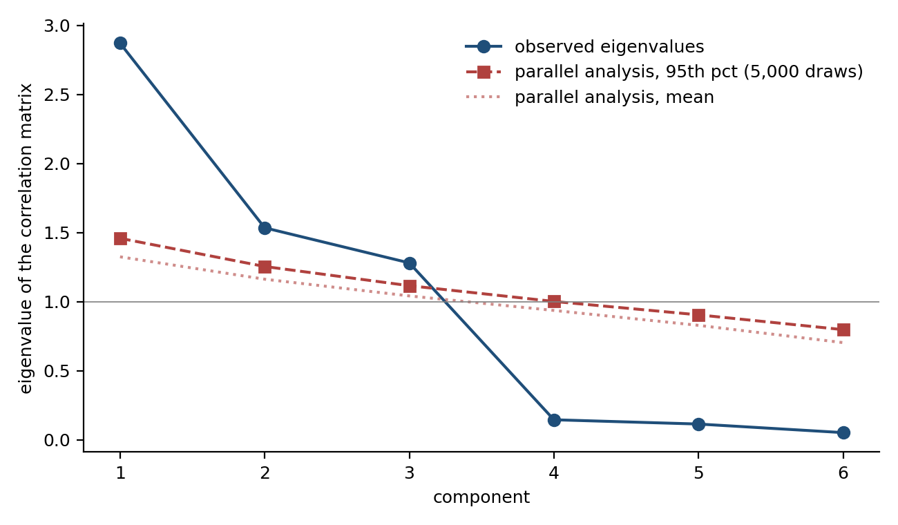
Parallel analysis retains three components on both the full and the reduced correlation matrix. The three explain 95% of the variance of the six measures (47%, 24% and 23%); the fourth eigenvalue, 0.15, is far below its permutation reference of 1.00 (Figure 1).
| Measure | C1 Local peg stability | C2 Supply trajectory | C3 Supply volatility | Communality |
|---|---|---|---|---|
peg_mad |
0.98 | 0.03 | 0.02 | 0.96 |
peg_p99 |
0.97 | 0.01 | 0.07 | 0.95 |
price_vol |
0.96 | 0.03 | 0.05 | 0.92 |
growth |
0.01 | -0.73 | 0.64 | 0.95 |
supply_vol |
0.08 | 0.15 | 0.96 | 0.96 |
max_drawdown |
0.06 | 0.95 | 0.23 | 0.96 |
Signs are as stated: higher C1 is a less stable price around local par, higher C2 is a supply path with a larger drawdown and lower growth, higher C3 is more variable supply. The promax solution is congruent with the varimax solution at 0.995 or above on every component, the principal-axis solution at 0.999 or above, and the bootstrap loadings at a median of 0.997 (fifth percentile 0.994).
Two features of the table matter for the rest of the note. First, the three price measures are one dimension: level, tail and dynamics correlate at 0.89 to 0.94 on a 180-day window, and the separation of chronic imprecision from episodic severity that the first version of this note reported does not exist once threshold replicates of the same series are removed. Second, growth loads on two components, against drawdown on C2 and with volatility on C3, so C2 reads as the direction of the supply path and C3 as its roughness. The Kaiser-Meyer-Olkin measure is 0.55 overall and below 0.3 for the three supply measures, which is to say the supply measures share little variance with each other: the components are close to the measures themselves, and the space is best read as three near-orthogonal coordinates rather than as latent factors.
5. No partition satisfies the rule
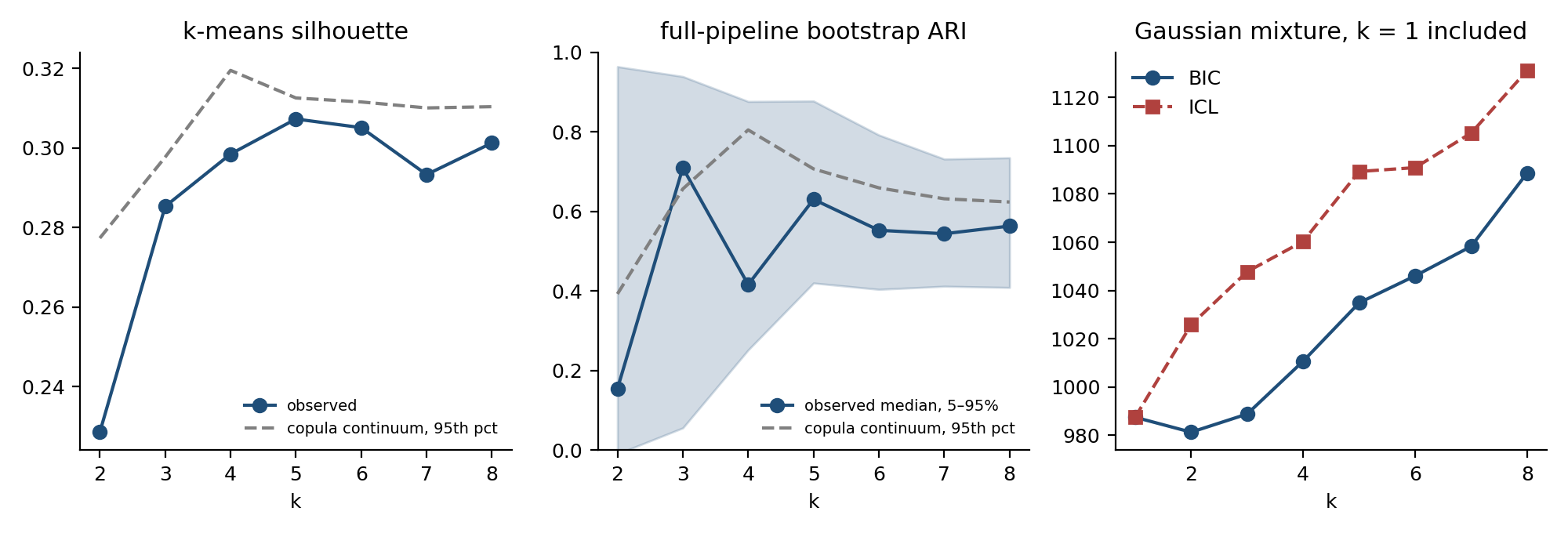
Table 3 and Figure 2 give the k-means partitions with their continuum references. The Monte Carlo interval on each cutoff is the 2.5th to 97.5th percentile of the cutoff over 200 bootstrap resamples of the 1,000 continuum draws that define it.
| k | Silhouette | Continuum 95th pct [MC interval] | Group sizes | Bootstrap ARI, median [5th, 95th] | Continuum 95th pct [MC interval] | Ward ARI |
|---|---|---|---|---|---|---|
| 2 | 0.229 | 0.277 [0.273, 0.283] | 46, 65 | 0.15 [-0.01, 0.96] | 0.39 [0.36, 0.42] | 0.00 |
| 3 | 0.285 | 0.298 [0.296, 0.299] | 48, 39, 24 | 0.71 [0.06, 0.94] | 0.66 [0.63, 0.67] | 0.33 |
| 4 | 0.298 | 0.319 [0.317, 0.323] | 44, 24, 21, 22 | 0.42 [0.25, 0.88] | 0.80 [0.78, 0.82] | 0.55 |
| 5 | 0.307 | 0.313 [0.311, 0.316] | 19, 31, 23, 21, 17 | 0.63 [0.42, 0.88] | 0.71 [0.69, 0.72] | 0.48 |
| 6 | 0.305 | 0.312 [0.309, 0.315] | 27, 19, 16, 25, 7, 17 | 0.55 [0.40, 0.79] | 0.66 [0.65, 0.67] | 0.38 |
| 7 | 0.293 | 0.310 [0.307, 0.312] | 14, 17, 22, 19, 10, 7, 22 | 0.54 [0.41, 0.73] | 0.63 [0.62, 0.64] | 0.42 |
| 8 | 0.301 | 0.310 [0.309, 0.313] | 16, 22, 13, 20, 3, 19, 10, 8 | 0.56 [0.41, 0.73] | 0.62 [0.61, 0.63] | 0.44 |
The six diagnostics read as follows.
Clustering tendency. Hopkins against a single Gaussian is 0.59; the copula continuum gives 0.56 and planted three-group mixtures 0.58 at a separation of three and 0.67 at four. The data are somewhat more concentrated than a Gaussian, as skewed marginals make them; the statistic does not separate the data from a mixture at three and does not reach a mixture at four.
Mixture criteria. BIC selects two components, by six points over one; the integrated completed likelihood, which charges for overlap, selects one by 39 points. Under the copula continuum BIC selects more than one component in 8.9% of draws and the integrated completed likelihood in 0.4%; under planted mixtures BIC selects more than one in 53% of draws at a separation of three and in every draw at four, the integrated completed likelihood in 15% and 99%. BIC prefers a two-component density fit, of the kind a continuum yields roughly one time in eleven; the integrated completed likelihood and the separation diagnostics do not support reading the fitted components as separated groups.
Gap statistic. One group under the uniform, the Gaussian and the copula reference. As stated in Section 3, the statistic selected one group in every simulated mixture as well, so it discriminates nothing at this sample size and dimension and carries no weight.
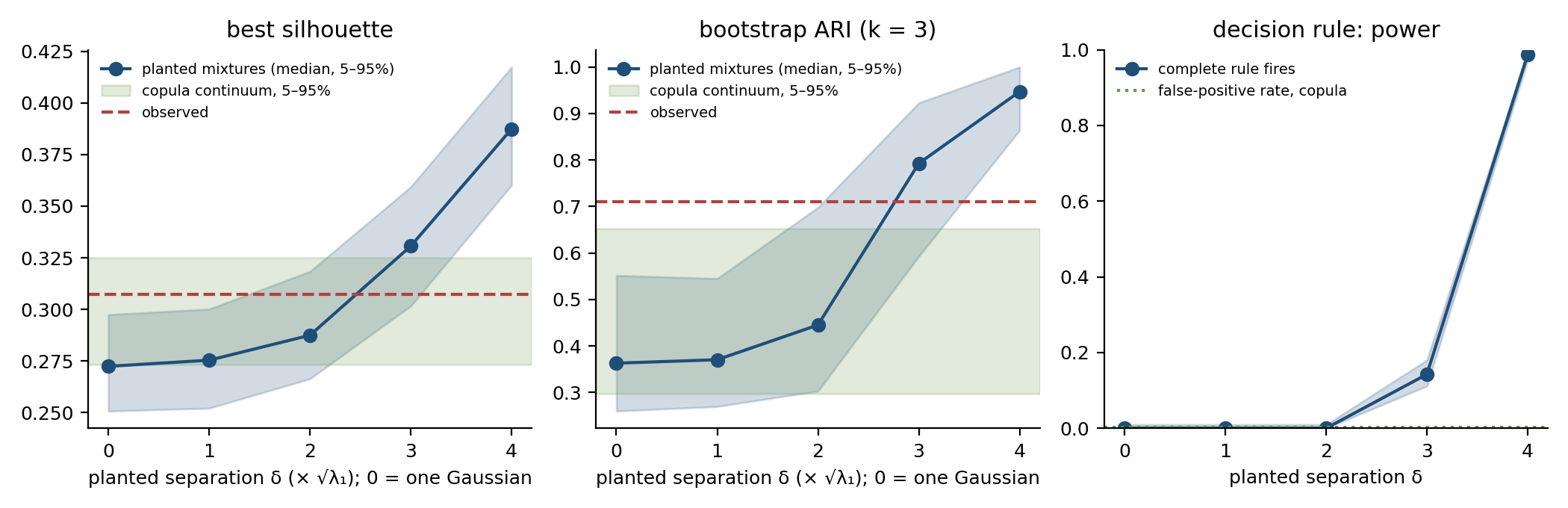
Silhouette. Between 0.23 and 0.31 at every k, below the continuum's 95th percentile at every k (Table 3), and below the lower end of each cutoff's Monte Carlo interval. Planted mixtures reach a best silhouette of 0.33 at a separation of three and 0.39 at four.
Method agreement. Ward's method recovers the k-means partition at an adjusted Rand index between 0.00 and 0.55.
Bootstrap stability. The full-pipeline bootstrap gives a median index of 0.71 at k = 3, with a 5th percentile of 0.06: across resamples the procedure returns either the same partition or a substantially different one. The continuum's 95th percentile at k = 3 is 0.66, with a Monte Carlo interval of 0.63 to 0.67, so the observed value exceeds the cutoff; this is the only statistic at any k that does (Figure 3, center). At every other k the observed median lies below its cutoff. Planted mixtures separated by three standard deviations give 0.79 at k = 3, by four 0.95. The k = 3 partition is driven by the supply block (a supply-only clustering of the same coins agrees with it at an index of 0.51, a price-only clustering at -0.01) and peels off the 24 coins whose supply fell most in the first six months (median drawdown 1.5 log points) from the rest. Fifteen of the 24 entered the record above $10 million, against 37 of the other 87, so the tail is in part coins that appear in the record already large and then shrink; on the coins whose record begins below $10 million the tail's k = 3 stability falls to 0.29 (Appendix C). Its stability is evidence on its own, and nothing else corroborates it: its silhouette is inside the continuum band and neither mixture criterion supports a partition. A tail of a skewed distribution reappears under resampling without being separated from its body.
The rule. On the observed data the rule does not fire: the bootstrap band is exceeded at k = 3 only, the silhouette band at no k, and the integrated completed likelihood selects one component. Under the continuum the rule fires in 0.2% of the 1,000 held-out draws (Wilson interval 0.1% to 0.7%) and in none of 400 single-Gaussian draws; under planted mixtures it fires in none of 400 draws at separations of one or two, in 14% at three (11% to 18%) and in 99% at four (97% to 99.5%). The calibration therefore bounds what the negative excludes: three groups separated by four standard deviations of the leading component would have been found in 99 of 100 such samples, three groups separated by three in 14 of 100, and groups separated by two or less in none. The rule is conservative by construction, since it requires four diagnostics to agree; types separated by three standard deviations or less remain possible and would not usually be recoverable from 111 coins by these methods.
Sensitivities. Appendix C gives the full diagnostic block for every variant; the variants were not separately calibrated, so their statistics are reported without cutoffs. On the loading-weighted scale BIC, the integrated completed likelihood and the gap statistic retain their primary selections (two, one and one) while k-means returns materially different partitions (agreement with the primary near zero at k = 2 and 3); a 200-resample full-pipeline bootstrap on that scale gives a median index of 0.70 at k = 3. The complete decision rule was not recalibrated on the loading-weighted scale. On the rank-transformed measures both mixture criteria select one component. With the 41 origin-unreliable coins added back and on the 96 dollar-pegged coins alone, the mixture and gap selections match the primary specification. The integrated completed likelihood selects two components in four variants: the unclipped measures, either measurement block alone, and the wider supply-only universe; in each the k = 3 bootstrap index is 0.35 to 0.80 and the best silhouette 0.315 to 0.362. Under the first version's log(1 + x) transform, which leaves the price measures with skewness of 4.6 to 5.8, both mixture criteria select two components and the partition is a different one (agreement with the primary 0.23 at k = 3); that transform did not tame the skew it was specified to tame, and its groups are the outliers it left in place.
6. Declared category and behavioral position
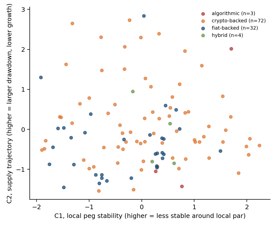
The launch backing label shifts the location of coins in the component space by a small and statistically detectable amount, and the dispersion test provides no evidence of a difference in spread (Figure 4): on the primary contrast of 72 crypto-backed against 32 fiat-backed coins the permutation pseudo-F is 4.21 (p = 0.006) and the label explains 4.0% of the variance of the scores, while a permutation test of the two groups' dispersion around their centroids does not reject equality (p = 0.84). Residualizing on log supply at day 179 and cohort year leaves 3.9% (p = 0.007). By component, fiat-backed coins sit 0.39 standard deviations below the mean on local peg stability against 0.12 above for crypto-backed (eta-squared 0.05, Holm-adjusted p = 0.040) and 0.37 below on supply trajectory against 0.18 above (eta-squared 0.07, Holm-adjusted p = 0.019); no difference in supply volatility is detected (p = 0.86). On the loading-weighted scale the global result is the same (pseudo-F 5.61, p = 0.005, 5.2% of variance).
A shift of location can still be a usable signal. The fully out-of-fold balanced accuracy of predicting the two labels from the six measures is 0.64 (range across 20 repetitions 0.57 to 0.68) against a chance level of 0.50 and a permutation 95th percentile of 0.60 (p = 0.010). Behavior in the first six months identifies the backing type better than a coin toss and far from reliably. With the seven hybrid and algorithmic launches pooled into a third class the global test weakens (4.5% of variance, p = 0.020), the per-component effects no longer survive the Holm adjustment (adjusted p = 0.053 and 0.058), and prediction does not exceed its permutation reference (0.39 against 0.33, p = 0.24); with three algorithmic launches in the universe, the analysis says nothing about that category. Descriptively, the three algorithmic launches sit 0.91 standard deviations above the mean on local peg stability.
Death shares by k-means group at k = 3 are 21% (10 of 48), 21% (8 of 39) and 42% (10 of 24), with Wilson intervals of [12%, 34%], [11%, 36%] and [24%, 61%]; the third group is the high-drawdown tail of Section 5. By launch label they are 31% (22 of 72, interval [21%, 42%]) for crypto-backed and 12.5% (4 of 32, interval [5%, 28%]) for fiat-backed coins. They are reported as description: the groups are tails of one distribution, the intervals overlap, and the mortality paper in preparation is where survival is modeled.
7. What the note establishes
Among well-documented stablecoins that survive a common early-life window, three statements hold. Early-life conduct is summarized by three near-orthogonal coordinates: local peg stability, supply trajectory and supply volatility. Under a stated rule with a measured false-positive rate, no partition of the coordinate space is jointly more separated, more model-supported and more stable than calibrated continuum references; under the planted-mixture design the rule fired in 99% of simulations at a separation of four standard deviations of the leading coordinate, in 14% at three, and in none of the 400 simulations at one or two. The declared backing category shifts a coin's expected position by a small amount, mostly on local price stability and supply trajectory for fiat-backed coins, and identifies the category only modestly.
For analysis and supervision the operational consequence is a preference for coordinates over classes within this population: a coin is better described by its position on the three axes than by membership in a behavioral group, because no grouping met the criterion this note set, and the one grouping that came closest is a tail of the supply-trajectory axis rather than a region separated from it.
8. Limitations
Coin identity was checked, not assumed: each coin's supply and price come from two providers joined on an identity crosswalk, and for the 107 primary coins whose supply provider publishes its own identifier for the price provider, that identifier agrees with the crosswalk in every case (262 agreements and no disagreement across the wider panel); the four remaining pairings rest on documented manual verification, one of them at medium confidence (VUSD). The estimand is conditional. The primary universe is 111 coins that survived 180 days and were observed through them with adequate coverage; they are larger and less mortal than the 200 excluded, and a type of coin that fails within its first six months cannot appear (the 90-day window in Appendix B admits eight more of the early deaths and still excludes 12; it relaxes the condition rather than removing it). The window is the first six months in the issuance record, which for coins that enter the record large is not the first six months of life; conduct later in life, and its change over time, is not examined. The origin clock is the record's first sustained $1 million, bounded but not curated coin by coin, and the sensitivity on coins whose record begins small (Appendix C) is the check on it. Par is estimated from the coin's own price, so the price measures describe stability, not fidelity to a promise. Feed artefacts were checked rather than assumed absent: no supply series in any window shows a fall of more than 90% that reverses within three days, so no rapid-reversal feed artefact of this kind explains the high-drawdown tail; two single-day price prints (MKUSD in the 180-day and 90-day windows, DJED in the 365-day window) are the only isolated artefacts found, they affect one coin's price-volatility measure in the primary window, neither coin sits in a tail group, and removing them leaves every diagnostic unchanged (Appendix C). The calibration plants Gaussian groups that share the empirical covariance, with centers on a simplex in the plane of the two leading eigenvectors; other geometries, and mixtures of unequal size, were not simulated, and the rule's power against them is unknown. The cutoffs that the rule uses are estimates with the Monte Carlo intervals shown in Table 3; at partition sizes where an observed statistic falls inside a cutoff's interval, the rule's verdict at that size is not sharp.
Data and code availability
The feature matrix, signed loadings, component scores with partition labels, all diagnostics for every window and sensitivity, the calibration draws' summaries, the selection flow and the analysis code are deposited with this note under its DOI, https://doi.org/10.5281/zenodo.23124313, as a replication package. Inputs are frozen at the issuance and price extracts of 19 July 2026 and the identity crosswalk and death registry of 30 July 2026. The raw daily series are the providers' and are not redistributed; the package carries the derived feature matrix, from which every result reproduces with the seeds recorded in the code and in each diagnostics file.
References
Anderson, M.J. (2001): "A new method for non-parametric multivariate analysis of variance", Austral Ecology, 26(1), 32–46.
Anderson, M.J. (2006): "Distance-based tests for homogeneity of multivariate dispersions", Biometrics, 62(1), 245–253.
Arner, D.W., R. Auer and J. Frost (2020): "Stablecoins: risks, potential and regulation", BIS Working Papers, No 905.
Bartlett, M.S. (1950): "Tests of significance in factor analysis", British Journal of Statistical Psychology, 3(2), 77–85.
Biernacki, C., G. Celeux and G. Govaert (2000): "Assessing a mixture model for clustering with the integrated completed likelihood", IEEE Transactions on Pattern Analysis and Machine Intelligence, 22(7), 719–725.
Bullmann, D., J. Klemm and A. Pinna (2019): "In search for stability in crypto-assets: are stablecoins the solution?", ECB Occasional Paper Series, No 230.
Fabrigar, L.R., D.T. Wegener, R.C. MacCallum and E.J. Strahan (1999): "Evaluating the use of exploratory factor analysis in psychological research", Psychological Methods, 4(3), 272–299.
Fraley, C. and A.E. Raftery (2002): "Model-based clustering, discriminant analysis, and density estimation", Journal of the American Statistical Association, 97(458), 611–631.
Gadzinski, G., A. Castello and F. Mazzorana (2023): "Stablecoins: does design affect stability?", Finance Research Letters, 53, 103611.
Hafner, M., M. Henriques Pereira, H. Dietl and J. Beccuti (2024): "The four types of stablecoins: a comparative analysis", Ledger, 9.
Hendrickson, A.E. and P.O. White (1964): "Promax: a quick method for rotation to oblique simple structure", British Journal of Statistical Psychology, 17(1), 65–70.
Hennig, C. (2007): "Cluster-wise assessment of cluster stability", Computational Statistics and Data Analysis, 52(1), 258–271.
Horn, J.L. (1965): "A rationale and test for the number of factors in factor analysis", Psychometrika, 30(2), 179–185.
Hubert, L. and P. Arabie (1985): "Comparing partitions", Journal of Classification, 2(1), 193–218.
Kaiser, H.F. (1958): "The varimax criterion for analytic rotation in factor analysis", Psychometrika, 23(3), 187–200.
Kaiser, H.F. (1974): "An index of factorial simplicity", Psychometrika, 39(1), 31–36.
Kwon, Y., K. Pongmala, K. Qin, A. Klages-Mundt, P. Jovanovic, C. Parlour, A. Gervais and D. Song (2023): "What drives the (in)stability of a stablecoin?", arXiv, 2307.11754.
Lawson, R.G. and P.C. Jurs (1990): "New index for clustering tendency and its application to chemical problems", Journal of Chemical Information and Computer Sciences, 30(1), 36–41.
Lorenzo-Seva, U. and J.M.F. ten Berge (2006): "Tucker's congruence coefficient as a meaningful index of factor similarity", Methodology, 2(2), 57–64.
Mizrach, B. (2025): "Stablecoins: survivorship, transactions costs, and exchange microstructure", The Journal of Alternative Investments, 27(4), 82–109.
Rousseeuw, P.J. (1987): "Silhouettes: a graphical aid to the interpretation and validation of cluster analysis", Journal of Computational and Applied Mathematics, 20, 53–65.
Steinley, D. (2004): "Properties of the Hubert-Arabie adjusted Rand index", Psychological Methods, 9(3), 386–396.
Song, M. (2026): "Stablecoin typologies beyond fiat denomination: evidence from deep temporal clustering", Finance Research Letters, 110, 110622.
Tibshirani, R., G. Walther and T. Hastie (2001): "Estimating the number of clusters in a data set via the gap statistic", Journal of the Royal Statistical Society: Series B, 63(2), 411–423.
Suggested citation
Silenzi, Massimiliano (2026): "Are there behavioral types of stablecoins? A calibrated test for discrete structure in survivors' early-life conduct", SB Research Notes, No 1, October. Stablecoin Beat Research. https://doi.org/10.5281/zenodo.23124313
Appendix A. Analysis sequence and forking paths
An earlier version of this analysis (July 2026) computed thirteen measures on each coin's full observed life, truncated 30 days before a verified death, and clustered the scores of four rotated components. Its measurement windows depended on the outcome, its measures were repeated summaries of two series, and its diagnostics had no reference. It was withdrawn.
The present design was fixed on 27 September 2026 before the rebuilt analysis was run: fixed windows from the origin, exclusion of origin-unreliable coins, six measures one per construct, the structure diagnostics with their references, the full-pipeline bootstrap and the direct category tests. Decisions taken after results had been seen are these. The price-coverage rule was relaxed from 80% to two thirds of window days after the selection flow, and only the selection flow, showed the feed's two-day gaps failing coins on density rather than behavior; the universe rose from 80 to 111 coins. The Hopkins reference was changed from uniform to Gaussian after a unit test on simulated data. The transform was changed from log(1 + x) to log(x + 1e-4) after the first run of the pipeline showed the price measures still skewed above 5; that run had shown more apparent structure than the present one, so the change moved the result against the earlier version's conclusion, and the log(1 + x) run is reported in Appendix C. Symmetric clipping at the 2.5th and 97.5th percentiles was added after the skewness table of the second run showed three coins with administratively frozen supply seven standard deviations below the median; the unclipped run is reported. The gap statistic was removed from the decision rule after the calibration showed it had no power, with the observed results already seen; the verdict on the observed data is the same under both rules. The primary category contrast was narrowed from three classes to fiat-backed against crypto-backed, the dispersion test, the Holm adjustment and the out-of-fold refitting were added, and the return-scaling rule for missing price days was set from the observed gap distribution, all in response to external review and before results under the revised procedures were seen; the two-class out-of-fold prediction result, which the pooled three-class test had hidden, is reported as found. No estimate from the mortality paper enters this note.
Appendix B. The 90-day and 365-day windows
The same pipeline on days 0 to 89 and 0 to 364 after origin, with the calibration at half the primary's draw counts (1,000 continuum, 200 per planted separation). The 90-day window is the survivor-selection check: it admits eight coins that died between day 90 and day 179 and excludes 12 that died inside its own window, against 20 for the primary. The 365-day window intensifies the selection (41 died inside it).
| 90 days | 180 days (primary) | 365 days | |
|---|---|---|---|
| Primary universe (verified dead) | 112 (29) | 111 (28) | 86 (23) |
| Died inside the window | 12 | 20 | 41 |
| Components retained; variance | 3; 96% | 3; 95% | 3; 95% |
| Loading congruence with the 180-day solution | 0.998 or above | 0.995 or above | |
| Hopkins against a single Gaussian | 0.70 | 0.59 | 0.58 |
| BIC; ICL components | 2; 1 | 2; 1 | 1; 1 |
| Gap statistic (all three references) | 1 | 1 | 1 |
| Best silhouette (k) | 0.352 (8) | 0.307 (5) | 0.312 (7) |
| k at which the silhouette exceeds its continuum cutoff | 7, 8 | none | none |
| Bootstrap ARI at k = 3; continuum cutoff | 0.51; 0.74 | 0.71; 0.66 | 0.73; 0.61 |
| k at which the bootstrap ARI exceeds its cutoff | 8 | 3 | 3 |
| Decision rule fires | no | no | no |
| Rule false-positive rate, continuum | 1.2% | 0.2% | 0.0% |
| Rule detection rate, separation 3; 4 | 11%; 98.5% | 14%; 99% | 8%; 90% |
| Fiat vs crypto: variance explained; p | 2.9%; 0.026 | 4.0%; 0.006 | 4.5%; 0.011 |
| Dispersion test p | 0.55 | 0.84 | 0.28 |
| Components with Holm-adjusted p < 0.05 | none | C1, C2 | C2 |
| Out-of-fold balanced accuracy; p | 0.58; 0.12 | 0.64; 0.010 | 0.65; 0.020 |
| High-drawdown group at k = 3: n; death share | 16; 50% | 24; 42% | 28; 46% |
Three readings. First, the component structure is the same at every horizon: three components, the three price measures on one, congruence with the primary loadings above 0.995 on every component. Second, the rule fires in none of the three windows. At 90 days the silhouette exceeds its cutoff at k = 7 and 8 and the bootstrap index at k = 8, in partitions whose smallest groups hold four or five coins, while the overlap-penalized mixture criterion selects one component; the continuum reference is also looser at 90 days, where BIC selects more than one component in 59% of continuum draws and the rule's own false-positive rate is 1.2%. At 365 days both mixture criteria select one component and the rule's false-positive rate is zero in 500 draws, with detection at a separation of four falling to 90% on 86 coins. Third, the high-drawdown group that k-means peels off at k = 3 is present in every window, with a death share of 42% to 50% against 14% to 28% in the other k = 3 groups, and is separated in none of them. The 90-day window relaxes the survivor condition and admits eight deaths excluded by the 180-day design, but still excludes the 12 coins that died inside 90 days; it shows the same high-drawdown tail, but its k = 3 stability remains below the 90-day continuum cutoff and no separation criterion supports it. The category shift is weakest at 90 days (no component survives the Holm adjustment, prediction at chance) and clearest at 365, where it sits on supply trajectory (eta-squared 0.10, Holm-adjusted p = 0.015) with out-of-fold balanced accuracy 0.65.
Appendix C. Sensitivity matrix
Every variant runs the applicable full pipeline (transform, extraction, rotation, scores, structure tests, and a 200-resample full-pipeline bootstrap); except for the loading-weighted row, component scores are standardized to unit variance. The variants were not separately calibrated; the primary cutoffs (Table 3) do not transfer to a different transform, feature block or universe, so the statistics stand without reference bands. Agreement is the adjusted Rand index between the variant's k = 3 partition and the primary's on the same coins.
| Variant | n | BIC k | ICL k | Gap k (copula) | Best silhouette (k) | Bootstrap ARI, k = 3 | Agreement with primary, k = 3 |
|---|---|---|---|---|---|---|---|
| Primary (log, clipped, unit-variance scores) | 111 | 2 | 1 | 1 | 0.307 (5) | 0.71 | 1.00 |
| Loading-weighted scores (Z L) | 111 | 2 | 1 | 1 | 0.366 (2) | 0.70 | -0.02 |
| Rank transform | 111 | 1 | 1 | 1 | 0.340 (6) | 0.63 | 0.66 |
| Unclipped | 111 | 3 | 2 | 1 | 0.315 (7) | 0.35 | 0.18 |
| Inherited log(1 + x) transform | 111 | 2 | 2 | 1 | 0.422 (2) | 0.71 | 0.23 |
| Supply block only, same coins | 111 | 3 | 2 | 1 | 0.362 (4) | 0.43 | 0.51 |
| Price block only, same coins | 111 | 2 | 2 | 1 | 0.320 (3) | 0.80 | -0.01 |
| Dollar-pegged coins only | 96 | 2 | 1 | 1 | 0.312 (7) | 0.82 | 1.00 |
| Origin-unreliable coins added back | 152 | 2 | 1 | 1 | 0.314 (4) | 0.80 | different universe |
| Supply block, wider universe | 167 | 3 | 2 | 1 | 0.349 (4) | 0.56 | different universe |
| Isolated price prints removed (one coin affected) | 111 | 2 | 1 | 1 | 0.305 (5) | 0.72 | 1.00 |
| Record begins below $50 million at origin | 93 | 1 | 1 | 1 | 0.302 (5) | 0.63 | 0.71 |
| Record begins below $10 million at origin | 59 | 1 | 1 | 1 | 0.321 (5) | 0.29 | 0.63 |